When you learn new technology, it's common to hear "don't worry about the low-level details--use the tools!" That's a good long-term strategy, but when you learn the lower-level details of how the tools work, it gives you a fuller understanding of what they can do for you. I decided to go through Andrew Trask's A Neural Network in 11 lines of Python to really learn how every line worked, and it's been very helpful. I had to review some matrix math and look up several numpy function calls that he uses, but it was worth it.
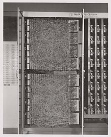
My title here refers to it as a "modern neural network" because while neural nets have been around since the 1950s, the use of backpropagation, a sigmoid function and the sigmoid's derivative in Andrew's script highlight the advances that have made neural nets so popular in machine learning today. For some excellent background on how we got from Frank Rosenblatt's 1957 hard-wired Mark I Perceptron (pictured here) to how derivatives and backpropagation addressed the limitations of these early neural nets, see Andrey Kurenkov's A 'Brief' History of Neural Nets and Deep Learning, Part 1. The story includes a bit more drama than you might expect, with early AI pioneers Marvin Minsky and Seymour Papert convincing the community that limitations in the perceptron model would prevent neural nets from getting very far. I also recommend Michael Nielsen's Using neural nets to recognize handwritten digits, in particular the part on perceptrons, which gives further background on that part of Kurenkov's "Brief History," and then Nielsen's sigmoid neurons part that follows it and describes how these limitations were addressed.
Andrew's 11-line neural network, with its lack of comments and whitespace, is more for show. The 42-line version that follows that is easier to follow and includes a great line-by-line explanation. Below are some of my own additional notes that I made as I dissected and played with his code. Often, I'm just restating something he already wrote but in my own words to try to understand it better. Hereafter, when I refer to his script, I mean the 42-line one.
I took his advice of trying the script in an IPython (Jupyter) notebook, where it was a lot easier to change some numbers (for example, the number of iterations in the main for loop) and to add print statements that told me more about what was happening to the variables through the training step iterations. After playing with this a bit and reviewing his piece again, I realized that many of my experiments were things that he suggests in his bulleted list that begins with "Compare l1 after the first iteration and after the last iteration." That whole list is good advice for learning more about how the script works.
Beneath his script and above his line-by-line description he includes a chart explaining each variable's role. As you read through the line-by-line description, I encourage you to refer back to that chart often.
I have minimal experience with the numpy library, but based on the functions from Andrew's script that I looked up, it seems typical that if you take a numpy function that does something to a number and pass it a data structure such as an array or matrix filled with numbers, it will do that thing to all the numbers and return the data structure.
Line 23 of Andrew's script initializes the weights that tell the neural net how much attention to pay to the input at each neuron. Ultimately, a neural net's job is to tune these weights based on what it sees in how input (in this script's case, the rows of X) corresponds to output (the values of y) so that when it later sees new input it will hopefully output the right things. When this script starts, it has no idea what values to use as weights, so it puts random values in, but not completely random--as Andrew writes, they should have a mean of 0. The np.random.random((x,y)) function returns a matrix of x rows of y random numbers between 0 and 1, so 2*np.random.random((3,1)) returns 3 rows with 1 number each between 0 and 2, and the "- 1" added to that makes them random numbers between -1 and 1.
np.dot() returns dot products. I found the web page How to multiply matrices (that is, how to find their dot product) helpful in reviewing something I hadn't thought about in a while. You can reproduce that page's "Multiplying a Matrix by a Matrix" example using numpy with this:
matrix1 = np.array([[1,2,3],[4,5,6]])
matrix2 = np.array([[7,8],[9,10],[11,12]])
print(np.dot(matrix1,matrix2))
The four lines of code in Andrew's main loop perform three tasks:
predict the output based on the input (
l0) and the current set of weights (syn0)check how far off the predictions were
use that information to update the weights before proceeding to the next iteration
If you increase the number of iterations, you'll see that first step get closer and closer to predicting an output of [[0][0][1][1]] in its final passes.
Line 29 does its prediction by calculating the dot product of the input and the weights and then passing the result (a 4 x 1 matrix like [[-4.98467345] [-5.19108471] [ 5.39603866] [ 5.1896274 ]], as I learned from one of those extra print statements I mentioned) to the sigmoid function named nonlin() that is defined at the beginning of the script. If you graphed the values potentially returned by this function, they would not fall in a line (it's "nonlinear") but along an S (sigmoid) curve. Looking at the Sigmoid function Wikipedia page shows that the expression 1/(1+np.exp(-x)) that Andrew's nonlin() function uses to calculate the function's return value (if the optional deriv parameter has a value of False) corresponds to the formula shown near the top of the Wikipedia page. This nonlin() function takes any number and returns a number between 0 and 1; as Andrew writes, "We use it to convert numbers to probabilities." For example, if you pass a 0 to the function (or look at an S curve graph) you'll see that the function returns .5; if you pass it a 4 or higher it returns a number very close to 1, and if you pass it a -4 or lower it returns a number very close to 0. The np.exp() function used within that expression calculates the exponential of the passed value--or all the values in an array or matrix, returning the same data structure. For example, np.exp(1) returns the natural logarithm e, which is about 2.718.
Line 29 calls that function and stores the returned matrix in the l1 variable. Reviewing the variable chart, this is the "Second Layer of the Network, otherwise known as the hidden layer." Line 32 then subtracts the l1 matrix from y (the array of answers that it was hoping to get) and stores the difference in l1_error. (Subtracting matrices follows the basic pattern of np.array([[5],[4],[3]]) - np.array([[1],[1],[1]]) = np.array([[4],[3],[2]]).)
Remember how line 23 assigned random values to the weights? After line 32 executes, the l1_error matrix has clues about how to tune those weights, so as the comments in lines 34 and 35 say, the script multiplies how much it missed (l1_error) by the slope of the sigmoid at the values in l1. We find that slope by passing l1 to the same nonlin() function, but this time, setting the deriv parameter to True to get that slope. (See "using the derivatives" in Kurenkov's A 'Brief' History for an explanation of why derivatives played such a big role in helping neural nets move beyond the simple perceptron models.) As Andrew writes, "When we multiply the 'slopes' by the error, we are reducing the error of high confidence predictions" (his emphasis). In other words, we're putting more faith in those high confidence predictions when we create the data that will be used to update the weights.
The script stores the result of multiplying the error by the slope in the l1_delta variable and then uses the dot product of that and l0 (from the variable table: "First Layer of the Network, specified by the input data") to update the weights stored in syn0.
Per Harald Borgen's Learning How To Code Neural Networks (which begins with an excellent description of the relationship of a neuron's inputs to its weights and goes on to talk about how useful Andrew's "A Neural Network in 11 lines of Python" is) says that backpropagation "essentially means that you look at how wrong the network guessed, and then adjust the networks weights accordingly." When someone on Quora asked Yann LeCun (director of AI research at Facebook and one of the Three Kings of Deep Learning) "Which is your favorite Machine Learning Algorithm?" his answer was a single eight-letter word: "backprop." Backpropagation is that important to why neural nets have become so fundamental in so many modern computer applications, so the updating of syn0 in line 39 is very crucial here.
And that's it for the neural net training code. After the first iteration, the weighting values in syn0 will be a bit less random, and after 9,999 more iterations, they'll be a lot closer to where you want them. I found that adding the following lines after line 29 gave me a better idea of what was happening in the l1 variable at the beginning and end of the script's execution:
   if (iter < 4 or iter > 9997):
        print("np.dot(l0,syn0) at iteration " + str(iter) + ": " + str(np.dot(l0,syn0)))
        print("l1 = " + str(l1))
(One note for people using Python 3, like I did: in addition to adding the parentheses in calls to the print function, the main for loop had to say just "range" instead of "xrange". More on this at stackoverflow.)
These new lines showed that after the second iteration, l1 had these values, rounded to two decimal place here: [[ 0.26] [ 0.36] [ 0.23] [ 0.32 ]]. As Andrew's output shows, at the very end, l1 equals [[ 0.00966449] [ 0.00786506] [ 0.99358898] [ 0.99211957]], so it got a lot closer to the [0,0,1,1] that it was shooting for. How can you make it get even closer? By increasing the iteration count to be greater than 10,000.
For some real fun, I added the following after the script's last line, because if you're going to train a neural net on some data, why not then try the trained network (that is, the set of tuned weights) on some other data to see how well it performs? After all, Andrew does write "All of the learning is stored in the syn0 matrix."
X1 = np.array([ [0,1,1], [1,1,0], [1,0,1],[1,1,1] ])
x1prediction = nonlin(np.dot(X1,syn0))
print(x1prediction)
The first two rows of my new input are different from those in the training data. The xlprediction variable ended up as [[ 0.00786466] [ 0.9999225 ] [ 0.99358931] [ 0.99211997]], which was great to see. Rounded, these are 0, 1, 1, and 1, so the neural net knew that for those first two rows of data--which it hadn't seen before--the output should be the first value from each.
Everything I describe here is from part 1 of Andrew's exposition, "A Tiny Toy Network." Part 2, "A Slightly Harder Problem" has a script that is eight lines longer (four lines if you don't count white space and comments) and I plan to dig into that next, because among other things, it has a more explicit demo of backpropagation.
Please add any comments to this Google+ post.
Image courtesy of Wikipedia.

